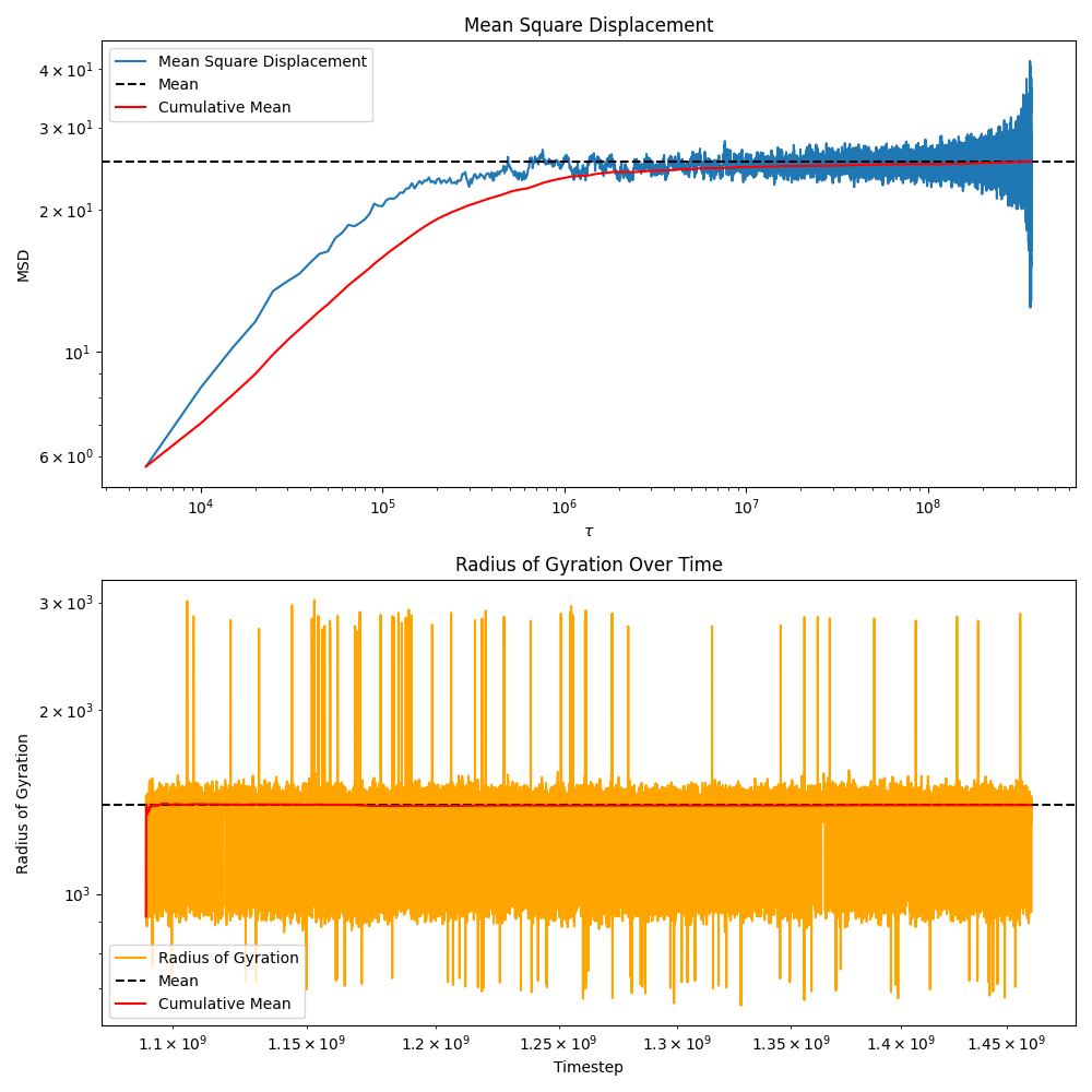
Trajectory Analysis

This example demonstrates how to analyze a polymer trajectory using pylimer-tools, including mean square displacement (MSD) and radius of gyration calculation.

import os

import matplotlib.pyplot as plt
import numpy as np

from pylimer_tools_cpp import UniverseSequence

# Load a LAMMPS dump trajectory file (replace with your file)
file_path = os.path.join(
    os.getcwd(),
    "../..",
    "tests/pylimer_tools/fixtures/",
)
sequence = UniverseSequence()
sequence.initialize_from_dump_file(
    initial_data_file=os.path.join(file_path, "big_dump_file_data.out"),
    dump_file=os.path.join(file_path, "big_dump_file.lammpstrj"),
)

# Compute the mean square displacement for all atoms
msd = sequence.compute_msd_for_atoms(
    atom_ids=[a.get_id() for a in sequence[0].get_atoms()],
    nr_of_origins=50,  # Number of origins to use for MSD calculation
)

You can also compute other properties like radius of gyration, end-to-end distance, etc. by using the “lazy” iterator over the sequence This allows you to process large trajectories without loading everything into memory at once.

# Compute radius of gyration over time
rgs = []
timesteps = []
for universe in sequence:
    rgs.append(
        np.mean(
            [
                m.compute_radius_of_gyration()
                for m in universe.get_molecules(
                    -1
                )  # -1 because we don't have any crosslinks to filter out
            ]
        )
    )
    timesteps.append(universe.get_timestep())

# Create a two-panel plot: MSD and Rg
fig, axs = plt.subplots(2, 1, figsize=(10, 10), sharex=False)

# Panel 1: MSD
axs[0].plot(
    list(
        msd.keys()), list(
            msd.values()), label="Mean Square Displacement")
axs[0].axhline(
    np.mean(
        list(
            msd.values())),
    color="black",
    linestyle="--",
    label="Mean")
# add cumulative mean
axs[0].plot(
    list(msd.keys()),
    [np.mean(list(msd.values())[: i + 1]) for i in range(len(msd))],
    label="Cumulative Mean",
    color="red",
)
axs[0].set_xlabel("$\\tau$")
axs[0].set_ylabel("MSD")
axs[0].set_title("Mean Square Displacement")
axs[0].set(xscale="log", yscale="log")
axs[0].legend()

# Panel 2: Radius of Gyration
axs[1].plot(timesteps, rgs, label="Radius of Gyration", color="orange")
axs[1].axhline(np.mean(rgs), color="black", linestyle="--", label="Mean")
# add cumulative mean
axs[1].plot(
    timesteps,
    [np.mean(rgs[: i + 1]) for i in range(len(rgs))],
    label="Cumulative Mean",
    color="red",
)
axs[1].set_xlabel("Timestep")
axs[1].set_ylabel("Radius of Gyration")
axs[1].set_title("Radius of Gyration Over Time")
axs[1].set(xscale="log", yscale="log")
axs[1].legend()

plt.tight_layout()
plt.show()

Please beware that the MSD is computed in an \(N^2\) manner, which can be slow for large systems, many origins and long trajectories.

If you want more origins or otherwise better performance, consider using the tidynamics package instead like so:

import tidynamics

# using sorted atom ids to make sure the order is consistent
# across all timesteps, which is important for MSD calculation
sorted_atom_ids = sorted([a.get_id() for a in sequence[0].get_atoms()])
msd_result = tidynamics.msd(
      np.array(
          [
              [
                  coord
                  for id in sorted_atom_ids
                  for coord in u.get_atom_by_vertex_id(id).get_coordinates()
              ]
              for u in sequence
          ]
    )
 )