Dissipative Particle Dynamics (DPD) Simulations

This example demonstrates how to set up and run a DPD simulation with slip-springs using pylimer-tools.

References: Langeloth et al. [LMBohmMullerPlathe13] and Schneider et al. [SFKarimiVarzanehMullerPlathe21].

Assuming your pylimer_tools version was compiled with OpenMP, to run this in parallel, you can use the typical OpenMP environment variables, e.g., in the terminal before running your script: export OMP_NUM_THREADS=4 to use 4 threads.

import os

import pandas as pd

from pylimer_tools.io.read_lammps_output_file import read_data_file
from pylimer_tools_cpp import (
    AtomStyle,
    ComputedDoubleValues,
    ComputedIntValues,
    DPDSimulator,
    OutputConfiguration,
)

# Load a LAMMPS data file (replace with your file)
filePath = os.path.join(
    os.getcwd(),
    "../..",
    "tests/pylimer_tools/fixtures/structure/melt_83_a_100.structure.out",
)
universe = read_data_file(
    filePath, atom_style=[AtomStyle.HYBRID, AtomStyle.BOND, AtomStyle.EDPD]
)

# Create the DPD simulator
dpd_simulator = DPDSimulator(
    universe=universe,
    seed="12345",  # Set a random seed for reproducibility*
)

Note that the random seed does not guarantee the same results across different runs, as the DPD algorithm is inherently stochastic and will produce different results if you use more than one processor.

# Randomly sample slip-springs
dpd_simulator.create_slip_springs(num=100)

# Configure what to output during the simulation on each step
step_output_config = OutputConfiguration()
step_output_config.int_values = [
    ComputedIntValues.STEP,  # Output the simulation step
]
step_output_config.double_values = [
    ComputedDoubleValues.TEMPERATURE,  # Output the temperature
    ComputedDoubleValues.PRESSURE,  # Output the pressure
    ComputedDoubleValues.STRESS_XX,  # Output the xx component of the stress tensor
    ComputedDoubleValues.STRESS_YY,  # Output the yy component of the stress tensor
    ComputedDoubleValues.STRESS_ZZ,  # Output the zz component of the stress tensor
]
step_output_config.output_every = 10  # Output every 10 steps
# temporary filename for output
step_output_config.filename = "dpd_simulation_output.txt"
dpd_simulator.config_step_output([step_output_config])

# Configure what to average during the simulation
avg_output_config = OutputConfiguration()
avg_output_config.int_values = [
    ComputedIntValues.STEP,  # Output the simulation step
]
avg_output_config.double_values = [
    ComputedDoubleValues.TEMPERATURE,  # Output the temperature
    ComputedDoubleValues.PRESSURE,  # Output the pressure
]
avg_output_config.output_every = 10
step_output_config.use_every = 1
avg_output_config.filename = "dpd_simulation_avg_output.txt"
dpd_simulator.config_average_output([avg_output_config])

dpd_simulator.run_simulation(
    n_steps=1000,  # Number of simulation steps
    dt=0.01,  # Time step size
    with_MC=True,  # Enable Monte Carlo moves of slip-springs
)

print("DPD simulation completed.")

DPD simulation completed.

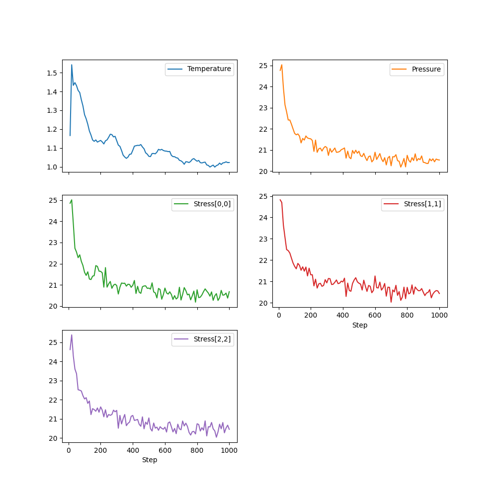
read the output file and actually plot something

df = pd.read_csv("dpd_simulation_output.txt", sep="\\s+")
_ = df.plot(
    x="Step",
    y=[
        "Temperature",
        "Pressure",
        "Stress[0,0]",
        "Stress[1,1]",
        "Stress[2,2]",
    ],
    subplots=True,
    layout=(3, 2),
    figsize=(10, 10),
)